In this post, I will concisely summarize my research study, “A study of data and label shift in the LIME framework,” which was a collaboration with my supervisor, Professor Henrik Boström. The paper was accepted as oral in the Neurips 2019 workshop on “Human-Centric Machine Learning.” You can read the paper on Arxiv, and the workshop website can be accessed here: https://sites.google.com/view/hcml-2019.
Introduction
In 2019, LIME explanations were prevalent [1], but LIME operated differed significantly from how explanations functioned in the older days. Before LIME, feature importance explanations were the weights of an interpretable model, and they were one vector that provided importance scores for all instances. LIME operated differently and could provide feature importance for a single instance $x$. LIME calls this to be a local explanation. To obtain Local LIME explanations, we need a black-box prediction function that outputs probability scores, $f$, and a background dataset that is usually the training set $X$. So far, so good. But there are three steps where things start to get complicated:
The first step is that LIME transforms the explained instance $x$ into an interpretable representation. For tabular datasets, this interpretable representation is a binary representation based on binning the feature values into the dataset into quartiles. For text datasets, the bag-of-words representation and the super-pixel representation are used for images.
The second step is when LIME randomly samples features present in the explained instances $x$ (features with zero value are omitted). For the case of text and image datasets, Each generated sample receives one; otherwise, its value is 0. Tabular datasets are a bit more complicated. A random number between one and four is generated for each randomly selected feature. If the explained instance $X$ has a feature with a corresponding value in the generated bin number, the value of that feature becomes one and zero otherwise. You can read more about this process in [2].
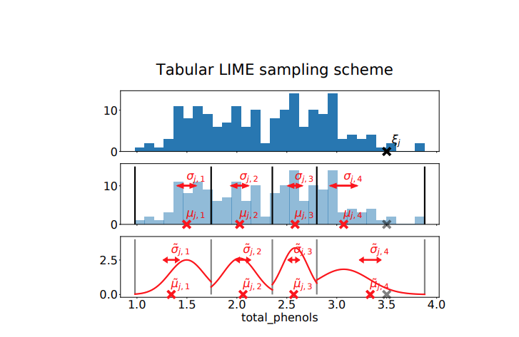
The third step is to transform these instances from binary to actual values. LIME replaces the values of the original explained instance with the values that received 1 in the text and image case. For tabular, it replaces the value that is between the selected quartile. This process is done $T$ times to obtain a sample $Z$. The sampling process for the Tabular dataset is shown in the figure taken from [2]:
The fourth and last step is that the LIME uses black-box prediction on these newly generated instances and learns a ridge regression model between the $(Z, f(Z))$ where $f(Z)$ is obtained with respect to a label $C$. Before training, each generated sample is weighted using a kernel function based on its proximity to the explained instance and passed to the Ridge model. After training the Ridge model, the weight of this Ridge regression model is the output local explanation.
Research Question
LIME claims that the weights of this Ridge model can show the important features in the vicinity (neighborhood) of the explained instance $x$. However, we suspected that the samples of $X$ and $Z$ might be too different, and the notion of vicinity might not apply between the neighboring instances of $x$ in $X$ and $Z$ samples. We wanted to investigate whether the nearest neighbors of $X$, $X_{\textrm{local}}$, and the samples of $Z$ come from the same distribution. Moreover, we wanted to investigate the same question for the predicted values of $f(Z)$ and $f(X_{\textrm{local}})$
Motivational Example
Let us see an example to show what we want to do. We train a Random Forest model on the third and fourth features of the Iris dataset. We’d like to highlight our question for the local explanations of test instance number ten in the Iris dataset. We set the number of LIME samples to 20.
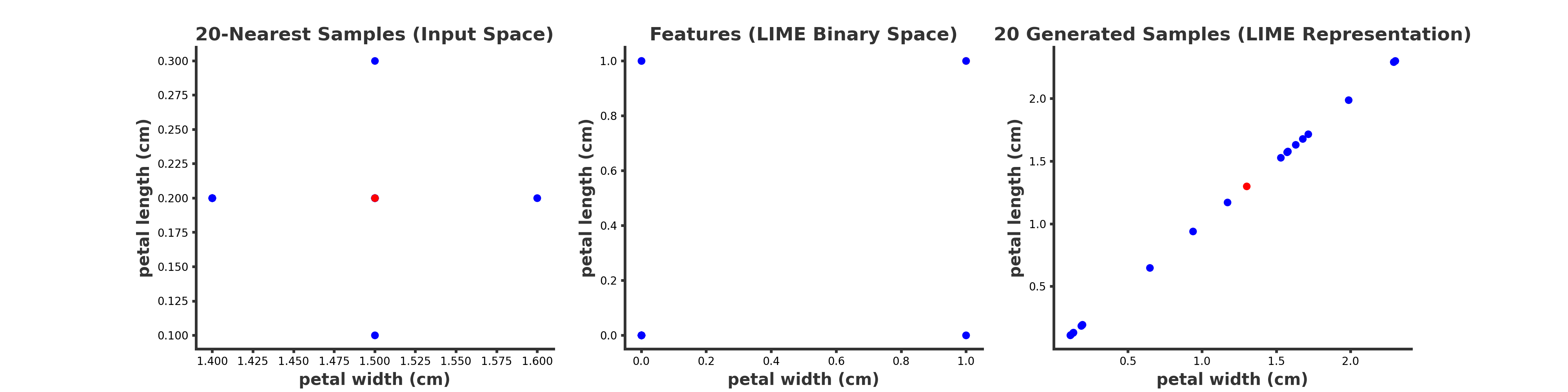
On the left, we see the explained instance (red dot) with 20 samples that are its nearest neighbors in the original input space $X$, namely $X_{\textrm{local}}$. In the middle, we see the intermediate binary sampled features. Since we are in 2-D, they are either (0,0), (0, 1), (1,0) or (1, 1). On the right hand, we see the explained instance and its samples transformed back into the LIME’s real space. Again, the red dot is the explained instance. Notice that the instance is shifted on the right figure since each feature value is set to the average values of its quartiles.
We can see the difference between these two spaces in these visualizations. The samples in the vicinity of the explained instance in the original input space (left) are very different from those in the LIME space (right).
Method
We could not just look at visualization. We needed a metric to measure this difference conclusively. Because of this, we used a two-sample Maximum Mean Discrepancy (MMD) test proposed in [3]. Like all other statistical tests, the MMD test provides us with a p-value and significance but also outputs the magnitude of the shift. Moreover, this test was reliable for samples with high feature dimensions. We ran the kernel test between the samples of the LIME explanations for each test instance $Z$ with its K-nearest neighbors in the original input space, $X_{\textrm{local}}$. In this comparison, naturally, $|Z| = |X_{\textrm{local}}| = n$. We set the acceptance level to be $\alpha=0.05$. The null hypothesis $H_0$ is that $P(Z) = P(X_{\textrm{local}})$. In other words, both come from the same distribution.
Evalution
Document Classification
The first use case is document classification using SVM models in the newsgroup dataset. This is one of the datasets investigated in the original LIME paper [1]. We obtained LIME explanations of each test instance for its predicted label and used the MMD two-sample test. In the Table below, you can see the results for explaining all test instances. In total, there are 717 test instances in the test dataset. Given the sampling size of $n$ for LIME, we can see that most of these samples diverge from their nearest neighbors in the original input space even in a small number of samples. The average and standard deviation of MMD values show significant divergence, especially for $n \geq 20$.
| $n$ | Reject | Failed to Reject | MMD |
|---|---|---|---|
| 2 | 417 (57%) | 300 (43%) | 0.42 ± 0.34 |
| 20 | 717 (100%) | 0 (0%) | 5.56 ± 1.58 |
| 100 | 717 (100%) | 0 (0%) | 24.77 ± 8.00 |
| 200 | 717 (100%) | 0 (0%) | 44.20 ± 15.84 |
| 500 | 717 (100%) | 0 (0%) | 87.35 ± 36.75 |
Image Classification
We performed a similar analysis for a subset of 100 test instances in ImageNet with the pre-trained InceptionV1 model. For the sample to be representative, we ensured that this subsample covers a large set of predicted classes. In this case, we found the nearest neighbors in the embedding space, as KNN suffers for high dimensional datasets. The table below shows the result for the ImageNet use case. We can see that the divergence is more significant for this case than in the previous case.
| $n$ | Reject | Failed to Reject | MMD |
|---|---|---|---|
| 50 | 188 (100 %) | 188 (0%) | 6.56 ± 0.13 |
| 100 | 188 (100 %) | 0 (0%) | 13.16 ± 0.20 |
| 200 | 188 (100 %) | 0 (0%) | 26.21 ± 0.35 |
| 500 | 188 (100 %) | 0 (0%) | 65.32 ± 0.67 |
We performed a similar analysis for the distribution of the predicted values for $P_{f(Z)}$ versus $P_{f(X_local)}$. The results can be found in Tables 2 and 4 in the paper.
Summary and conclusion
Our study showed a divergence between the LIME samples of the explained instances versus those near the explained instance in the original data space. Our empirical study questions whether, as LIME claimed in its original paper, the explanation from the Ridge surrogate model contains information about the vicinity of the explained instance.
We conclude that random sampling without restriction is not a suitable method to obtain explanations. One possible fix is to avoid transforming the instances and perform the sampling in the original input space. This was later investigated in [4], but the authors did not compare their results to the original LIME method. We also propose that using a decision tree surrogate can fix the problem with LIME. This is because decision trees have a model-intrinsic way of showing locality by forming regions created by logical rules.
Citation
If you want to cite our work, please use the following Bibtex entry:
@article{rahnama2019study,
  title={A study of data and label shift in the LIME framework},
  author={Rahnama, Amir Hossein Akhavan and Bostr{\"o}m, Henrik},
  journal={NeurIPS 2019 Workshop of Human-Centric Machine Learning},
  year={2019}
}
References:
[1]: Ribeiro, Marco Tulio, Sameer Singh, and Carlos Guestrin. “Why should I trust you? Explaining the predictions of any classifier.” Proceedings of the 22nd ACM SIGKDD international conference on knowledge discovery and data mining. 2016.
[2]: Garreau, Damien, and Ulrike von Luxburg. “Looking deeper into tabular LIME.” arXiv preprint arXiv:2008.11092 (2020).
[3]: Gretton, Arthur, et al. “A kernel two-sample test.” The Journal of Machine Learning Research 13.1 (2012): 723-773.
[4]: Molnar, Christoph, Giuseppe Casalicchio, and Bernd Bischl. “iml: An R package for interpretable machine learning.” Journal of Open Source Software 3.26 (2018): 786.